One way to make your data legible is to apply cell shading to every
other row in a range. Excel's Conditional Formatting feature (available
in Excel or later) makes this a simple task.
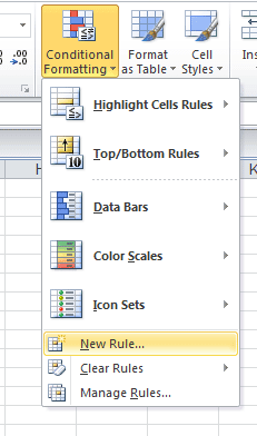
1. Select the range that you want to shade, then click Home>> Conditional Formatting>> New Rule... See screenshot:
2. Then a New Formatting Rule dialog box will pop out. Select Use a formula to determine which cells to format item. Then Input the formula “=MOD(ROW(),2)” in Format values where this formula is true.

3. Then click the Format… button, another Format Cells dialog box will pop out. Go to Fill tab and choose one colour for shading the background. See screenshot:

3. Click OK to return the New Formatting Rule dialog box, and also you will see the colour in the Preview box.
4. Then click OK. You will get the result you want. See screenshot:
 |  |
The best part is that the row shading is dynamic. You'll find that the
row shading persists even if you insert or delete rows within the
original range.
Notes:
1. Insert or delete a row in the shading range and you will see that the shading persists.
2. If you want to shade alternate columns,using this formula “=MOD(COLUMN(),2)”.
Download: Example of Alternate Row Shading


0 Comments